"So here is the thing, we want to have a list of values that the user can choose from in the cells of our sheet"

-Your boss

Dropdown lists of the sort shown below are very common and can be hugely beneficial for users when filling out Excel sheets. They are quite easy to create and offer basic data validation so that the user can't accidentally type in the wrong value.

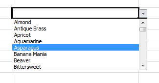
Lists with values can be very useful when creating data-entry sheets

TL;DR; If you just want to jump to the solution then feel free to download the demo sheet straight away :)

Demo File

But yeah, back to the data validation lists.

You can create one very easily via the ribbon through Data >> Data Validation

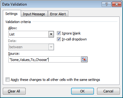
So easy...

Super!

"So yeah, this is great. But we want the list of values to be editable by the user."

-Your boss

Wait. That's easy! I can use ranges in these cell lists. So I'll just have one sheet that acts like a "Configuration" sheet and have some column in that sheet hold all the values to show in the list.

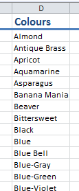
A list of colour names, so easy to add new ones at the end... so easy

Then I will just have the list pull data from a big chunk of the range so that the user can add items to the end of the list indefinately.

Oh my, still so easy...

Too many blanks

Unfortunately using an unbounded range for the list items causes a rather annoying bug. In the dropdown lists there will be a large section of completely empty items at the end. Even through you tick the Ignore blank option.

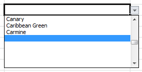
When using ranges a bunch of empty values appear at the end of the list. Annoying!

This is made even worse by the fact that the list always automatically scrolls down to the first blank item when entering values into an empty cell.

There are some solutions to this. Using the OFFSET function to limit the number of items in the list box is one of the fastest and simplest.

The OFFSET function can be used to help. But requires a lot of extra cells

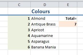
However to use the OFFSET function you need to know the total number of items to trim to, which requires you to use intermediate cells to count non-blank items. In the image above the green cells in column C count up when the cell in column D has a value. Then the cell orange cell in column E just takes the =MAX(C:C) range. This number you can use as the limit to the OFFSET function straight in the data validation box:

=OFFSET(Configuration!D2:D4000,0,0,Configuration!$E$3)

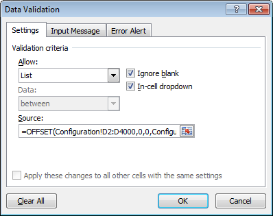
Data Validation using the OFFSET function

For some this is an acceptable solution. But for most this is just too brittle as the user might accidentally delete values in either column C or E and break the entire thing.

Read more about the OFFSET function on MSDN.

Too many items

Alright, no worries, you can fix this.

How about we use VBA to construct a simple string list of items and insert it directly into the cell validation list?

Something like this:

Public Function ApplyConfigLookupToRange(
                  applyToCells As Range, 
                  lookupValuesRange As Range)

  Dim ddl As String
  Dim Value As Variant
  For Each Value In lookupValuesRange
    If Value = "" Or IsEmpty(Value) Then
      'As soon as there is a blank entry in 
      'the list then exit, list must be contiguous
      Exit For 
    End If

    'Note: Regardless of the language/region set for Excel 
    'this feature always uses comma (,) as a separator
    ddl = ddl & Value & "," 
  Next Value

  'Trim the last comma from the end of the list
  If Len(ddl) > 0 Then
    ddl = Mid(ddl, 1, Len(ddl) - 1)
  End If

  'If there are no items to add to the list
  'then just delete everything from the range
  If Len(ddl) < 1 Then
    With applyToCells.Validation
        .Delete
    End With
  Else
    With applyToCells.Validation
        .Delete
        .Add Type:=xlValidateList, _
             AlertStyle:=xlValidAlertStop, _
             Operator:=xlBetween, _
             Formula1:=ddl
        .IgnoreBlank = True
        .InCellDropdown = True
    End With
  End If
End Function

Then we can simply call this function when we deactivate the Configuration sheet and apply it to our entire range. Something like so:

Private Sub Worksheet_Deactivate()
  Call ApplyConfigLookupToRange(
                Sheet1.Range("$A$1:$A$4000"),  ' All cells that should have the list dropdown
                "Configuration!$D$2:$D$4000")) ' List of colours
End Sub

Yes, this will work!

And it does, for a while...

Note: When specifying ranges like in the Worksheet_Deactivate function above. Always use the fully locked formula with $ signs for both columns and rows.

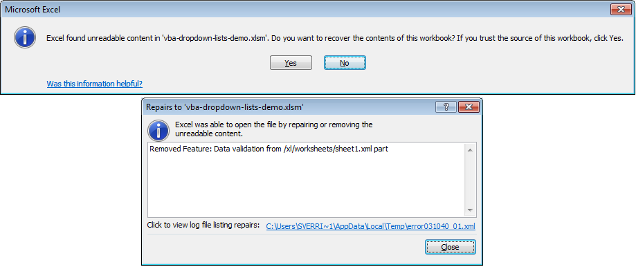
Error unreadable content in workbook

For a while the VBA solution works. But then suddenly your users start complaining about a strange error that keeps coming up when they open their sheet in the morning. They constantly have to have Excel "recover it" and when they do it seems that some content gets removed during repair.

They're worried!

Super scary errors, what did you remove! Tell me... WHAT!!

You can't find anything wrong with your code.

But the error is easily reproducible. There is something wrong. Everytime the sheet is closed and reopened the error appears.

You check, but the users really haven't deleted anything critical or messed with the formulas. They've just been adding more colours to the list as they were instructed to do and was a major selling point for them to use your Workbook.

Then you find it. Bam! There is an undocumented max-limit for string lists! They cannot be longer than 256 characters!

groan

So you cannot use your VBA solution after all. What to do?

Hybrids to the rescue

The real solution involves combining both of the approaches above in a way that circumvents the string limit of 256 characters while still keeping the sheet robust enough to handle users deleting rows willy-nilly without stuff breaking.

Tired? Want to jump to the solution?... Go ahead :)

Demo File

We modify our VBA code to produce an OFFSET function instead of a string. Then we make this function operate on the value range and places it in the data validation logic using VBA!

Like so:

Public Function ApplyConfigLookupToRange(
                  applyToCells As Range, 
                  lookupValuesRangeName As String)

  ' First we must count the values in the range
  Dim numItems As Long

  ' Now evaluate the range and loop through it 
  ' counting all of the consecutive values
  Dim lookupValuesRange As Range
  Set lookupValuesRange = Range(lookupValuesRangeName)
  For Each Value In lookupValuesRange
   If Value = "" Or IsEmpty(Value) Then
     Exit For
   End If
   numItems = numItems + 1
  Next Value

  ' Stop executing if nothing in the range
  If (numItems < 1) Then
   With applyToCells.Validation
      .Delete
    End With
  End If

  Dim formulaTemplate As String
  formulaTemplate = "=OFFSET(" + lookupValuesRangeName + _
                    ",0,0," + Str(numItems) + ")"

  ' Now create the drop-down validation boxes
  ' for the entire cell range that was passed in
  With applyToCells.Validation
      .Delete
      .Add Type:=xlValidateList, AlertStyle:=xlValidAlertStop, _
           Operator:=xlBetween, Formula1:=formulaTemplate
      .IgnoreBlank = True
      .InCellDropdown = True
  End With
End Function

The way we call the function is still the same

Private Sub Worksheet_Deactivate()
  Call ApplyConfigLookupToRange(
                ' Cells that should have the list dropdown
                Sheet1.Range("$A$1:$A$4000"),  
                ' List of all available colours
                "Configuration!$D$2:$D$4000")) 
End Sub

That's all there is too it. You circumvent the string limitation, keep the necessary elements for OFFSET out of the way of the user and have a list of values that the user can expand practically indefinitely.

fanfare!

Note on Named Ranges

I want to recommend the use of named ranges instead of the COL:ROW + $ pattern.

Named ranges are preferable as their extent can be modified without going behind the scenes to manipulate the raw VBA code. They also do not need any special $ handling to avoid a "shift" when generating the OFFSET functions and applying them to the cell ranges.

Managing the named ranges can then be done by non-programmers after the sheet is delivered to its users. In the example below I have replaced the hard-coded COL:ROW patterns with named ranges:

Private Sub Worksheet_Deactivate()
  Call ApplyConfigLookupToRange(
           Sheet1.Range("DataEntry_Colour_Cells"), 
           "List_Colour_Names")
End Sub

Read more about ranges on MSDN.

Note on calling the code

And where should I then call this code?

Ideally I think this code should be called directly on Worksheet_Deactivate when leaving the configuration sheet. That way the correct cells are always kept up to date after the user changes the list contents.

Now for the actual working demo, check it out!

Demo File

Happy coding!

• ← Newer
• Older →